Autoregressive Integrated Moving Average – ARIMA
The Autoregressive Integrated Moving Average (ARIMA) model is a widely used time series forecasting model that combines autoregression (AR), differencing (I for Integrated), and moving averages (MA) to capture various aspects of time series data. ARIMA is effective for modeling time series with trend and seasonality components.
Here’s an overview of the components and structure of the ARIMA model:
- Autoregressive (AR) Component (p): The AR component represents the relationship between the current value of the time series and its past values. It incorporates lagged values to capture autocorrelation. An AR(p) model uses ‘p’ past values.
- Integrated (I) Component (d): The I component represents differencing, which is applied to make the time series stationary. If the original time series is non-stationary (e.g., it has a trend), differencing is performed to remove the trend. The ‘d’ parameter indicates the number of differences required to achieve stationarity.
- Moving Average (MA) Component (q): The MA component models the relationship between the current value and past forecast errors. An MA(q) model uses ‘q’ past forecast errors.
The general form of an ARIMA model can be expressed as ARIMA(p, d, q):
Xt = c + ϕ1Xt−1 + ϕ2Xt−2 + … + ϕpXt−p – ϕ1ϵt−1 – ϕ1ϵt−2 – … – ϕqϵt−q + ϵt
- Xt is the value at time “t.”
- c is a constant or intercept.
- ϕ1, ϕ2, …, ϕp are the autoregressive coefficients.
- Xt−1, Xt−2, …, Xt−p are the lagged values.
- ϵt is the white noise or error term.
To use ARIMA for time series forecasting, you need to determine the appropriate values of ‘p,’ ‘d,’ and ‘q’ based on the characteristics of your data. This typically involves visual inspection of the data, ACF (AutoCorrelation Function) and PACF (Partial AutoCorrelation Function) plots, and statistical tests for stationarity (e.g., Augmented Dickey-Fuller).
Once you’ve determined the ARIMA order (p, d, q), you can fit the model to your time series data and use it for forecasting future values. Libraries like statsmodels in Python provide tools for ARIMA modeling and forecasting.
Here’s a simplified Python code snippet to fit and forecast with an ARIMA model:
import pandas as pd
import statsmodels.api as sm

# Load your time series data into a pandas DataFrame
# Replace this with your own time series data
# Example: data = pd.read_csv('your_data.csv')

# Fit an ARIMA model
model = sm.tsa.ARIMA(data, order=(p, d, q))
results = model.fit()

# Forecast future values
forecast = results.predict(start=len(data), end=len(data) + n-1, dynamic=False)
Replace p, d, q, and n with your chosen ARIMA order and the number of periods you want to forecast into the future. The forecast variable will contain the forecasted values.


