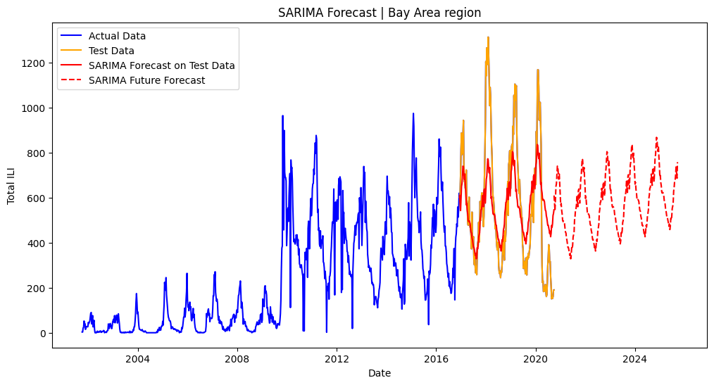
Seasonal Autoregressive Integrated Moving Average – SARIMA

The Seasonal Autoregressive Integrated Moving Average, or SARIMA, is an extension of the ARIMA model that is specifically designed to handle time series data with seasonality. SARIMA combines autoregression (AR), differencing (I for Integrated), moving averages (MA), and seasonal components. It’s a powerful model for forecasting time series data that exhibits both trend and seasonal patterns.

The SARIMA model is denoted as SARIMA(p, d, q)(P, D, Q, s), where:

• p is the order of the autoregressive component.
• d is the degree of differencing.
• q is the order of the moving average component.
• P is the seasonal autoregressive order.
• D is the seasonal differencing order.
• Q is the seasonal moving average order.
• s is the length of the seasonal cycle (e.g., 12 for monthly data, 7 for daily data with weekly seasonality).

Here’s a brief explanation of each component:

1. Autoregressive (AR) Component (p): It models the relationship between the current value and past values within a season.
2. Differencing (I) Component (d): It represents differencing, which is applied to make the time series stationary. The ‘d’ parameter indicates the number of differences required to achieve stationarity.
3. Moving Average (MA) Component (q): It models the relationship between the current value and past forecast errors within a season.
4. Seasonal Autoregressive (SAR) Component (P): It models the seasonal relationship between the current value and past values at the same season in previous years.
5. Seasonal Differencing (D) Component (D): It represents the seasonal differencing, which is applied to remove seasonality. The ‘D’ parameter indicates the number of seasonal differences.
6. Seasonal Moving Average (SMA) Component (Q): It models the seasonal relationship between the current value and past seasonal forecast errors.

The general form of a SARIMA model is:

Xt = c + ϕ1Xt−1 + … + ϕpXt−p - θ1ϵt−1 - ... - θqϵt−q - Φ1Xt−s - ... - ΦpXt−Ps + Θ1ϵt−s + ... + ΘQϵt−Qs + ϵt

This represents the components of an SARIMA model where:

• Xt is the value at time “t.”
• c is a constant or intercept.
• ϕ1, …, ϕp are the autoregressive coefficients.
• θ1, …, θq are the moving average coefficients.
• Φ1, …, Φp are the seasonal autoregressive coefficients.
• Θ1, …, Θq are the seasonal moving average coefficients.
• s is the length of the seasonal cycle (e.g., 12 for monthly data, 7 for daily data with weekly seasonality).
• Xt−1, Xt−2, …, Xt−p are the lagged values.
• ϵt is the white noise or error term.

Here’s a simplified Python code snippet to fit and forecast with an SARIMA model:

import pandas as pd
import statsmodels.api as sm

# Load your time series data into a pandas DataFrame
# Replace this with your own time series data
# Example: data = pd.read_csv('your_data.csv')

# Fit a SARIMA model
order = (p, d, q)
seasonal_order = (P, D, Q, s)
model = sm.tsa.SARIMAX(data, order=order, seasonal_order=seasonal_order)
results = model.fit()

# Forecast future values
forecast = results.get_forecast(steps=n)
forecast_mean = forecast.predicted_mean
forecast_confidence_intervals = forecast.conf_int()

Replace the following placeholders:

• p, d, q, P, D, Q, s: Replace these with your chosen SARIMA order parameters.
• data: Load your own time series data into a pandas DataFrame.
• n: Specify the number of periods you want to forecast into the future.

This code template should work once you’ve filled in the actual values. If you encounter specific errors while implementing the code with your data, please let me know the details, and I’ll be happy to assist further.